- E-mail:BD@ebraincase.com
- Tel:+8618971215294
Fiber photometry has become a widely used approach for monitoring neurotransmitter and calcium dynamics in vivo. However, for researchers new to the technique, interpreting raw traces and processing data can be challenging.
Questions such as distinguishing genuine biological signals from artifacts, selecting appropriate smoothing parameters, and handling baseline drift are common during early experiments. This article outlines a practical workflow for signal evaluation, artifact identification, and data processing in fiber photometry experiments.
One of the most common mistakes beginners make is confusing artifacts with biological signals.
A genuine neurotransmitter or calcium signal typically exhibits the following characteristics:
-The signal channel (470 nm) shows specific changes associated with behavioral events.
-The reference channel (405/410 nm) does not exhibit proportional synchronous changes.
-Stable responses remain after regression-based correction using the reference channel.
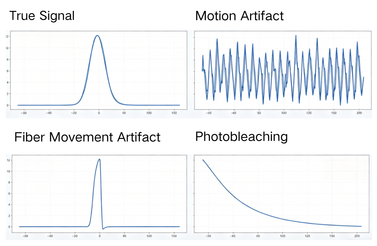
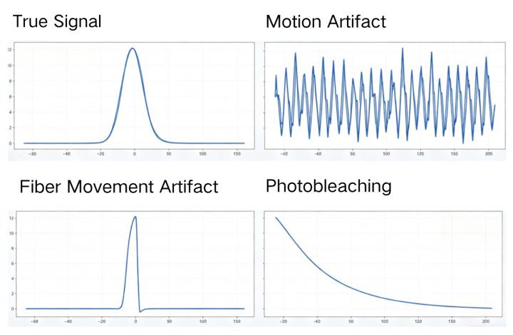
Figure 1. Representative examples of genuine signals and artifacts
Three Quick Rules for Identifying Real Signals
Real Signals
-The temporal dynamics should match the characteristics of the sensor and the behavioral event. For example, some neurotransmitter sensors rise within tens of milliseconds to 1 second and decay within 1–5 seconds.
-Signal waveforms are generally smooth and consistent. Minor spikes may appear in raw data but become more regular after appropriate smoothing.
Artifacts
-Characterized by abrupt jumps, sharp transitions, cliff-like rises or drops, or random fluctuations.
-Often show no meaningful relationship to behavioral events or experimental stimuli.
Photobleaching Is Not an Artifact
-Photobleaching is a common non-physiological baseline drift that should be corrected during data processing.
-A gradual, synchronized decline in both channels without sudden spikes is typically normal photobleaching.
Key Point
Highly synchronized changes in both channels often indicate non-specific influences such as movement, photobleaching, or hemodynamic effects, which require further correction and analysis.
| Artifact Type | Typical Signal Pattern | Cause | Recommended Solution |
|---|---|---|---|
| Motion Artifact | Complete synchronization between channels with no specific peaks | Animal movement, respiration, or body motion causing fiber displacement | Use flexible patch cords, include a reference channel (e.g., 405 nm), and account for movement-related effects during experimental design. |
| Fiber Movement / Displacement | Sudden baseline shifts and abrupt waveform changes | Fiber movement, loose connectors, or head scratching/twisting | Ensure secure ferrule connections and maintain stable positioning. |
| Normal Photobleaching | Gradual synchronized decline in both channels without spikes | Fluorophore photobleaching caused by laser excitation | Pre-bleach for 5–10 min, reduce excitation power, use more photostable sensors, and apply baseline correction. |
| Electrical Noise | Dense high-frequency spikes throughout the recording | Instrument electronics or photon detection noise | Verify grounding, isolate power supplies, and apply notch filtering when necessary. |
| Fluorescence Saturation | Signal clipped at upper or lower limits | Fluorescence exceeds detector dynamic range | Reduce excitation power, shorten exposure time, decrease gain, or lower expression levels. |
Raw fiber photometry recordings often contain high-frequency noise that can obscure underlying biological signals. Signal smoothing is therefore commonly applied to improve data visualization while preserving the temporal characteristics of genuine fluorescence responses.
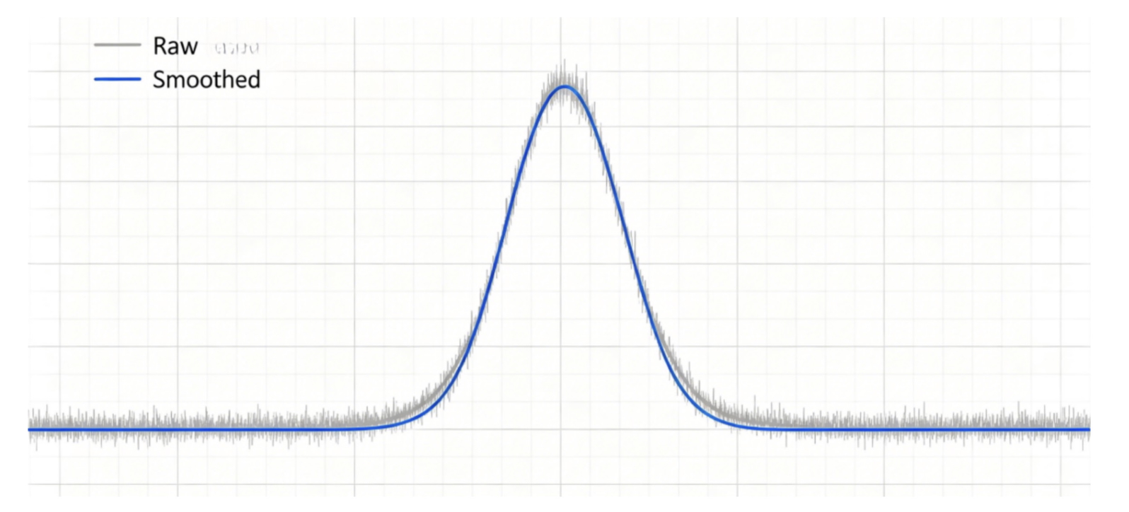
Figure 2. Comparison before and after signal smoothing
Before Smoothing
-Gray trace (raw signal): neurotransmitter peaks are visible but obscured by high-frequency noise and baseline fluctuations.
After Smoothing
-Blue trace (smoothed signal): high-frequency noise is removed while peak amplitude, rise time, and decay kinetics remain unchanged.
Several smoothing approaches are commonly used in fiber photometry data analysis. The choice of method depends on the recording quality, sampling rate, and the intended application.
Moving Average Filtering
Moving average filtering is widely used for routine data visualization and presentation purposes. It can be applied to both raw fluorescence traces and ΔF/F₀ signals. As a general guideline, a 9-point window is often suitable for data acquired at 20 Hz, while a 15-point window is commonly used for recordings acquired at 50 Hz. The optimal window size should be determined according to the sampling frequency, sensor kinetics, and the temporal features of interest.
Gaussian Smoothing
Gaussian smoothing is frequently used when preparing figures for publications because it produces smoother trace profiles while preserving overall signal dynamics. In most cases, a Sigma value between 2.0 and 3.0 provides satisfactory results, with other parameters remaining at their default settings.
Butterworth Low-Pass Filtering
Butterworth low-pass filtering is commonly used for quantitative analysis and more rigorous signal processing. A second-order filter with a cutoff frequency of 1.5 Hz is often suitable for neurotransmitter and calcium sensor recordings. The sampling frequency should be set according to the actual acquisition rate of the experiment.
Data Processing Considerations
Signal smoothing should be performed only after artifact correction and ΔF/F₀ calculation. A typical workflow includes reference-channel regression for artifact removal, followed by ΔF/F₀ calculation and subsequent smoothing.
Excessive smoothing should be avoided, as overly large smoothing windows or excessively low cutoff frequencies may attenuate biologically relevant fluorescence transients. In most cases, smoothing is applied to ΔF/F₀ traces rather than raw fluorescence signals. Raw fluorescence data should first undergo photobleaching correction and reference-channel fitting before downstream processing.
Origin provides several built-in smoothing functions that are widely used for fiber photometry data visualization. To perform smoothing, import the time series and ΔF/F₀ data into Origin and select the corresponding Y column. The smoothing tools can be accessed through:
Analysis → Signal Processing → Smooth
Origin supports multiple smoothing options, including Moving Average, Gaussian, and Butterworth filtering.
For Gaussian smoothing, a Sigma value of approximately 2.0 is commonly used. For Butterworth filtering, a second-order filter with a cutoff frequency of 1.5 Hz is often appropriate, although parameters may require adjustment depending on the characteristics of the recording.
After processing, Origin automatically generates a new curve while retaining the original dataset. Comparing the processed trace with the original signal is recommended to ensure that peak amplitude, rise time, and decay kinetics remain appropriately preserved.
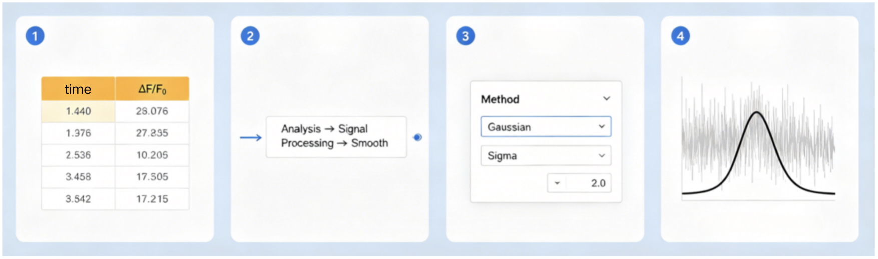
Figure 3. Example Origin workflow for signal smoothing
A typical fiber photometry analysis workflow consists of artifact assessment, signal normalization, noise reduction, and data visualization.
The first step is to evaluate recording quality and identify potential artifacts. The 410 nm reference channel can be used to assess motion-related interference, fiber movement, and other non-specific fluctuations. Recording segments affected by severe artifacts should be excluded from subsequent analysis.
Raw data are typically exported from the acquisition software in CSV, TXT, or MAT format. The exported dataset generally includes timestamps, the signal channel (470 nm), and the reference channel (410 nm).
After reference-channel correction and baseline fitting, fluorescence changes are commonly expressed as:
ΔF/F₀ = (F(t) − F₀) / F₀
where F₀ represents the average fluorescence intensity during a stable baseline period.
Following ΔF/F₀ calculation, appropriate filtering or smoothing can be applied to reduce high-frequency noise and improve signal visualization. Parameter selection should be based on the sampling frequency and the temporal characteristics of the sensor being used.
For data presentation and statistical analysis, both raw and processed traces should be retained whenever possible. Figures should clearly indicate analysis parameters and processing methods to ensure transparency and reproducibility. Depending on the experimental design, subsequent analyses may include event-aligned averaging, peak amplitude measurements, area-under-the-curve calculations, or other quantitative metrics.
Accurate fiber photometry analysis depends on proper artifact identification, reference-channel correction, and appropriate signal processing. Establishing a consistent analysis workflow can improve data quality and facilitate interpretation across experiments.
The Brain Case team will continue to share practical knowledge, insights, and experimental tips for reference purposes only. For inquiries about our products and services, please contact us at bd@ebraincase.com.


WhatsApp Business Account
Address:-
Address:-